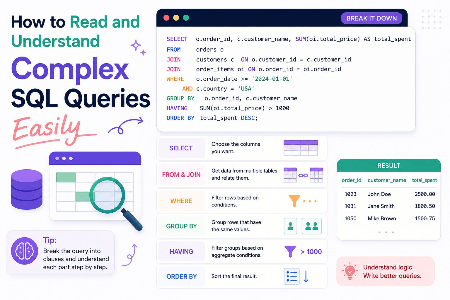
How to Read and Understand Complex SQL Queries Easily

A long SQL query can look intimidating when it contains several joins, nested expressions, aggregations, common table expressions, and window functions.

Fortunately, most complex queries are combinations of a small number of familiar operations:

• Select rows from one or more tables
• Match related records
• Filter unwanted rows
• Group records
• Calculate aggregate values
• Rank or compare rows
• Sort the result
• Limit the final output

The key is not to read every character from top to bottom. Instead, identify the query’s major stages and determine what each stage contributes to the final result.

This guide presents a repeatable method for analyzing complex SELECT queries safely and accurately.

Logical Processing vs Physical Execution

A SQL statement is written approximately like this:

SELECT ...
FROM ...
JOIN ...
WHERE ...
GROUP BY ...
HAVING ...
ORDER BY ...
LIMIT ...;

However, the clauses are easier to understand using a logical sequence closer to:

1. WITH
2. FROM
3. JOIN and ON
4. WHERE
5. GROUP BY
6. HAVING
7. Window-function calculations
8. SELECT
9. DISTINCT
10. Set operations such as UNION
11. ORDER BY
12. LIMIT or OFFSET

This is a conceptual model, not a guarantee of physical execution.

A database optimizer can:

• Reorder joins
• Push filters closer to table scans
• Choose an index
• Replace a subquery with a join
• Use a hash, merge, or nested-loop join
• Perform operations in parallel
• Eliminate unnecessary work

PostgreSQL, for example, documents the logical processing stages of SELECT, while its planner remains free to choose an efficient physical execution strategy.⁠⁠

Use the logical order to understand the result. Use the execution plan to understand how the database produces it.

A Quick Example

Consider this query:

SELECT
    c.id,
    c.name,
    COUNT(o.id) AS completed_order_count,
    SUM(o.total_amount) AS total_spent
FROM customers AS c
JOIN orders AS o
    ON o.customer_id = c.id
WHERE o.status = 'completed'
GROUP BY
    c.id,
    c.name
HAVING SUM(o.total_amount) >= 500
ORDER BY total_spent DESC
LIMIT 20;

It can be translated into plain language:

1. Start with customers and orders.
2. Match every order to its customer.
3. Keep only completed orders.
4. Group the remaining rows by customer.
5. Calculate each customer’s order count and total spending.
6. Keep customers who spent at least 500.
7. Sort them from highest to lowest spending.
8. Return the first 20 customers.

Once translated this way, the query becomes much easier to understand.

A Repeatable Method for Reading Any SQL Query

Step 1: Identify the Statement Type

Start by finding the query’s main operation.

Common statement types include:

• SELECT
• INSERT
• UPDATE
• DELETE
• MERGE
• CREATE
• ALTER

This guide focuses on SELECT, but the distinction matters because data-modification statements require extra caution.

A statement beginning with WITH may still be a SELECT, UPDATE, or DELETE.

Example:

WITH inactive_users AS (
    SELECT id
    FROM users
    WHERE last_login_at < CURRENT_DATE - INTERVAL '1 year'
)
DELETE FROM users
WHERE id IN (
    SELECT id
    FROM inactive_users
);

Do not assume a query is read-only merely because it starts with WITH.

Step 2: Format the Query

Never analyze a complex query as one continuous line.

Instead of:

SELECT c.name,SUM(o.total_amount) FROM customers c JOIN orders o ON o.customer_id=c.id WHERE o.status='completed' GROUP BY c.name;

Use:

SELECT
    c.name,
    SUM(o.total_amount) AS total_spent
FROM customers AS c
JOIN orders AS o
    ON o.customer_id = c.id
WHERE o.status = 'completed'
GROUP BY
    c.name;

Formatting reveals:

• Clause boundaries
• Join relationships
• Nested expressions
• Repeated calculations
• Missing conditions
• Alias usage

An SQL formatter or parser can help with unfamiliar queries, but always review the output. Different SQL dialects have different syntax.

Step 3: Find the Query’s Final Output

Although the SELECT list is not the first logical stage, it tells you what the query is trying to return.

Examine each selected expression:

SELECT
    c.id,
    c.name,
    COUNT(o.id) AS order_count,
    SUM(o.total_amount) AS total_spent

The output contains:

• One customer identifier
• One customer name
• A count of orders
• A total amount

This suggests that the result probably has one row per customer.

Write down the intended result shape:

One row per customer with completed-order count and total spending.

This statement becomes your hypothesis. The remaining clauses should confirm or contradict it.

Step 4: Identify Every Data Source

Now inspect:

• FROM
• JOIN
• CTEs
• Derived tables
• Views
• Table-valued functions

Example:

FROM customers AS c
JOIN orders AS o
    ON o.customer_id = c.id

Ask:

• Which table is the starting point?
• Which additional tables are joined?
• Are any names views rather than physical tables?
• Does a CTE transform the data before the main query?
• Are rows generated by a function?
• Does the same table appear more than once?

Create a quick source map:

For a large query, this small table can remove significant confusion.

Step 5: Understand Every Join

For each join, identify:

1. Join type
2. Left input
3. Right input
4. Matching condition
5. Expected relationship
6. Possible row multiplication

Example:

JOIN orders AS o
    ON o.customer_id = c.id

This appears to connect:

customers.id → orders.customer_id

The likely relationship is one customer to many orders.

That means one customer row may become several joined rows before grouping.

Ask the cardinality question

For every join, ask:

How many rows can this join create for one row from the left side?

Possible answers include:

• Zero
• One
• Many

This question is essential because joining two one-to-many relationships can multiply rows unexpectedly.

Example:

FROM customers AS c
JOIN orders AS o
    ON o.customer_id = c.id
JOIN support_tickets AS t
    ON t.customer_id = c.id

Suppose a customer has:

• Three orders
• Four support tickets

The joined result may contain:

3 × 4 = 12 rows

Aggregating this result without accounting for multiplication could overcount orders, tickets, or revenue.

Step 6: Recognize the Join Type

INNER JOIN

Returns matching rows from both sides.

FROM customers AS c
JOIN orders AS o
    ON o.customer_id = c.id

Customers without orders are excluded.

LEFT JOIN

Returns all rows from the left side and matching rows from the right.

FROM customers AS c
LEFT JOIN orders AS o
    ON o.customer_id = c.id

Customers without orders remain, with NULL in the order columns.

RIGHT JOIN

Returns all rows from the right side and matching rows from the left.

Many teams avoid RIGHT JOIN because reversing the table order and using LEFT JOIN is often easier to read.

FULL OUTER JOIN

Returns:

• Matched rows
• Unmatched left rows
• Unmatched right rows

CROSS JOIN

Produces every combination of rows.

FROM colors
CROSS JOIN sizes

If there are five colors and four sizes, the result contains 20 combinations.

An accidental cross join can create an enormous intermediate result.

Step 7: Separate Join Conditions from Row Filters

The difference between ON and WHERE is especially important with outer joins.

Consider:

SELECT
    c.id,
    o.id AS order_id
FROM customers AS c
LEFT JOIN orders AS o
    ON o.customer_id = c.id
WHERE o.status = 'completed';

Although this uses LEFT JOIN, the WHERE condition removes rows where o.status is NULL.

As a result, customers without completed orders disappear. The query behaves much like an inner join for that condition.

Compare it with:

SELECT
    c.id,
    o.id AS order_id
FROM customers AS c
LEFT JOIN orders AS o
    ON o.customer_id = c.id
   AND o.status = 'completed';

Now every customer remains, but only completed orders are matched.

When reading an outer join, always inspect later WHERE conditions involving the nullable side.

Step 8: Read the WHERE Clause as Row-Level Filtering

The WHERE clause removes individual rows before grouping.

Example:

WHERE
    o.status = 'completed'
    AND o.completed_at >= DATE '2026-01-01'
    AND c.deleted_at IS NULL

Translate each condition:

• Keep completed orders
• Keep orders completed in 2026 or later
• Exclude deleted customers

Pay attention to Boolean grouping

These conditions are not equivalent:

WHERE status = 'completed'
   OR status = 'refunded'
  AND total_amount > 100;

WHERE (
        status = 'completed'
        OR status = 'refunded'
      )
  AND total_amount > 100;

Because AND normally has higher precedence than OR, explicit parentheses improve safety and readability.

Check NULL comparisons

This is incorrect:

WHERE deleted_at = NULL

Use:

WHERE deleted_at IS NULL

SQL uses three-valued logic involving:

• TRUE
• FALSE
• UNKNOWN

Comparisons involving NULL commonly produce UNKNOWN, which can affect filtering in ways that surprise developers.

Step 9: Determine the Grouping Grain

When a query contains GROUP BY, identify what one result row represents.

Example:

GROUP BY
    c.id,
    c.name

The result is grouped by customer.

Another example:

GROUP BY
    c.id,
    DATE_TRUNC('month', o.completed_at)

Now one result row represents:

One customer in one month

This is the query’s grain.

Write it down explicitly.

Many SQL mistakes occur because developers misunderstand whether a row represents:

• One customer
• One order
• One customer per month
• One product per warehouse
• One event per day

Step 10: Understand Aggregate Functions

Common aggregate functions include:

• COUNT
• SUM
• AVG
• MIN
• MAX

Example:

SELECT
    c.id,
    COUNT(o.id) AS order_count,
    SUM(o.total_amount) AS total_spent
FROM customers AS c
JOIN orders AS o
    ON o.customer_id = c.id
GROUP BY c.id;

COUNT(*) vs COUNT(column)

These expressions are different:

COUNT(*)

Counts rows.

COUNT(o.id)

Counts rows where o.id is not NULL.

This matters with a LEFT JOIN.

Example:

SELECT
    c.id,
    COUNT(*) AS joined_row_count,
    COUNT(o.id) AS order_count
FROM customers AS c
LEFT JOIN orders AS o
    ON o.customer_id = c.id
GROUP BY c.id;

For a customer with no orders:

• COUNT(*) may return 1 because the customer’s outer-join row exists
• COUNT(o.id) returns 0 because o.id is NULL

Step 11: Read HAVING as Group-Level Filtering

WHERE filters rows before grouping.

HAVING filters groups after aggregation.

Example:

HAVING SUM(o.total_amount) >= 500

This means:

Keep only groups whose total order amount is at least 500.

Another example:

HAVING COUNT(o.id) >= 5

This means:

Keep only customers with at least five matching orders.

Do not mentally merge WHERE and HAVING. They operate at different stages.

Step 12: Understand Common Table Expressions

A common table expression, or CTE, creates a named intermediate result.

Example:

WITH completed_orders AS (
    SELECT
        id,
        customer_id,
        total_amount,
        completed_at
    FROM orders
    WHERE status = 'completed'
)
SELECT
    c.id,
    c.name,
    SUM(co.total_amount) AS total_spent
FROM customers AS c
JOIN completed_orders AS co
    ON co.customer_id = c.id
GROUP BY
    c.id,
    c.name;

Read it in two pieces.

CTE

completed_orders = all completed orders

Main query

Join customers to completed orders and calculate total spending.

Build a CTE dependency map

A complex query may contain several CTEs:

WITH
completed_orders AS (...),
customer_totals AS (...),
ranked_customers AS (...)
SELECT ...
FROM ranked_customers;

Map them as:

completed_orders
        ↓
customer_totals
        ↓
ranked_customers
        ↓
final result

This makes a large query resemble a sequence of smaller transformations.

Do not assume a CTE is always materialized as a temporary result. Optimizer behavior depends on the database, query, and CTE options.

Step 13: Handle Subqueries According to Their Type

“Always read the inner query first” works for some subqueries but not all.

Independent subquery

SELECT
    id,
    name
FROM customers
WHERE id IN (
    SELECT customer_id
    FROM orders
    WHERE total_amount > 1000
);

The inner query can be understood independently:

Find customer IDs associated with orders above 1,000.

The outer query then returns those customers.

Correlated subquery

SELECT
    c.id,
    c.name
FROM customers AS c
WHERE EXISTS (
    SELECT 1
    FROM orders AS o
    WHERE o.customer_id = c.id
      AND o.status = 'pending'
);

The subquery refers to c.id from the outer query.

Read it as:

For each customer, check whether at least one pending order exists for that customer.

A correlated subquery cannot be fully understood in isolation because it depends on the current outer row.

EXISTS vs IN

EXISTS asks whether a matching row exists.

WHERE EXISTS (
    SELECT 1
    FROM orders AS o
    WHERE o.customer_id = c.id
);

IN compares a value against a set:

WHERE c.id IN (
    SELECT o.customer_id
    FROM orders AS o
);

The optimizer may transform these into similar plans, but their NULL behavior and readability can differ.

Be especially careful with NOT IN when the subquery can return NULL. NOT EXISTS is often easier to reason about safely.

Step 14: Identify Window Functions

Window functions calculate values across related rows without collapsing those rows into one group.

Example:

SELECT
    o.id,
    o.customer_id,
    o.total_amount,
    ROW_NUMBER() OVER (
        PARTITION BY o.customer_id
        ORDER BY o.completed_at DESC
    ) AS order_position
FROM orders AS o;

Translate the window definition:

Within each customer, order records from newest to oldest and number them.

Unlike GROUP BY, this query still returns individual order rows.

Break the window into parts

Function

ROW_NUMBER()

Assigns a sequential number.

Partition

PARTITION BY o.customer_id

Restarts the numbering for each customer.

Ordering

ORDER BY o.completed_at DESC

Gives the newest order number 1.

Common window functions

• ROW_NUMBER
• RANK
• DENSE_RANK
• LAG
• LEAD
• FIRST_VALUE
• LAST_VALUE
• Windowed SUM
• Windowed AVG
• Windowed COUNT

Example running total:

SELECT
    account_id,
    transaction_date,
    amount,
    SUM(amount) OVER (
        PARTITION BY account_id
        ORDER BY transaction_date
        ROWS BETWEEN UNBOUNDED PRECEDING
                 AND CURRENT ROW
    ) AS running_balance
FROM transactions;

When a window frame is specified, inspect it carefully. The frame determines which surrounding rows contribute to the calculation.

Step 15: Find CASE Expressions

A CASE expression applies conditional logic.

SELECT
    id,
    total_amount,
    CASE
        WHEN total_amount >= 1000 THEN 'high'
        WHEN total_amount >= 500 THEN 'medium'
        ELSE 'standard'
    END AS order_tier
FROM orders;

Read it from top to bottom:

1. If amount is at least 1,000, label it high.
2. Otherwise, if amount is at least 500, label it medium.
3. Otherwise, label it standard.

The first matching branch wins.

A badly ordered CASE can make later conditions unreachable:

CASE
    WHEN total_amount >= 100 THEN 'large'
    WHEN total_amount >= 1000 THEN 'very large'
END

The second branch never applies because values above 1,000 already satisfy the first condition.

Step 16: Inspect DISTINCT

DISTINCT removes duplicate result rows after the selected expressions are evaluated.

SELECT DISTINCT
    customer_id
FROM orders;

This returns unique customer IDs.

When DISTINCT appears after several joins, ask why duplicates exist.

It may be:

• Intentionally returning unique values
• Hiding expected one-to-many expansion
• Masking an incorrect join
• Compensating for duplicated source data

Do not assume adding DISTINCT fixes a query. It may conceal a data-model or join problem.

Step 17: Understand Set Operations

SQL can combine query results using:

• UNION
• UNION ALL
• INTERSECT
• EXCEPT

Example:

SELECT email
FROM customers

UNION

SELECT email
FROM newsletter_subscribers;

UNION removes duplicate rows.

SELECT email
FROM customers

UNION ALL

SELECT email
FROM newsletter_subscribers;

UNION ALL preserves duplicates.

When reading a set operation, analyze each query independently before examining how the results are combined.

Confirm that corresponding columns have compatible meanings and data types.

Step 18: Read ORDER BY, LIMIT, and Pagination Last

Example:

ORDER BY total_spent DESC
LIMIT 20;

This returns the 20 highest values according to total_spent.

Check deterministic ordering

This may not be stable:

ORDER BY created_at DESC
LIMIT 20;

If several rows share the same timestamp, their relative order may vary.

A deterministic alternative is:

ORDER BY
    created_at DESC,
    id DESC
LIMIT 20;

Inspect OFFSET

LIMIT 20 OFFSET 10000;

This means the database must skip many earlier rows. Large offsets can be inefficient and can produce inconsistent pagination when records are added or removed between requests.

That is primarily a performance and API-design concern, but recognizing it helps explain the query’s purpose.

Step 19: Translate the Query into Plain Language

After inspecting all clauses, explain the query without SQL keywords.

For example:

Return the 20 customers who have spent at least 500 on completed orders since the beginning of 2026. Include each customer’s completed-order count and total spending, ordered from highest to lowest spending.

If you cannot describe the query clearly, revisit:

• Join cardinality
• Grouping grain
• Subquery dependencies
• NULL behavior
• Window partitions
• Filters on outer-joined tables

A good plain-language description should identify:

• The output grain
• The data sources
• The matching relationships
• The filters
• The calculations
• The sorting and limits

Complete Complex Query Example

Consider the following query:

WITH monthly_customer_spend AS (
    SELECT
        o.customer_id,
        DATE_TRUNC('month', o.completed_at) AS month,
        SUM(o.total_amount) AS total_spent
    FROM orders AS o
    WHERE o.status = 'completed'
      AND o.completed_at >= DATE '2026-01-01'
    GROUP BY
        o.customer_id,
        DATE_TRUNC('month', o.completed_at)
),
ranked_customers AS (
    SELECT
        mcs.customer_id,
        mcs.month,
        mcs.total_spent,
        DENSE_RANK() OVER (
            PARTITION BY mcs.month
            ORDER BY mcs.total_spent DESC
        ) AS spending_rank
    FROM monthly_customer_spend AS mcs
)
SELECT
    rc.month,
    rc.spending_rank,
    c.id AS customer_id,
    c.name,
    rc.total_spent
FROM ranked_customers AS rc
JOIN customers AS c
    ON c.id = rc.customer_id
WHERE rc.spending_rank <= 5
ORDER BY
    rc.month,
    rc.spending_rank,
    c.id;

Break it down

First CTE: monthly_customer_spend

For every customer and month, calculate spending from completed
orders during 2026.

Its grain is:

One row per customer per month.

Second CTE: ranked_customers

Within each month, rank customers by spending.

DENSE_RANK allows ties without gaps between later ranking values.

Main query

Join the ranked results to customer details, keep the top five
ranks for each month, and display the result in chronological and
ranking order.

Final description

For each month in 2026, show customers in the top five spending ranks based on completed orders.

This query is easier to understand as three transformations rather than one large statement.

How to Verify Your Interpretation

Reading is only the first step. Verify what you think the query does.

Inspect a small result

During development, temporarily select useful diagnostic columns:

SELECT
    c.id AS customer_id,
    o.id AS order_id,
    o.status,
    o.total_amount
FROM customers AS c
JOIN orders AS o
    ON o.customer_id = c.id
WHERE c.id = 101;

This can confirm whether joins and filters behave as expected.

Count rows between stages

Use CTEs to inspect intermediate counts:

WITH filtered_orders AS (
    SELECT *
    FROM orders
    WHERE status = 'completed'
)
SELECT COUNT(*)
FROM filtered_orders;

Test known examples

Choose records for which the expected result can be calculated manually.

Include cases such as:

• Customer with no orders
• Customer with one order
• Customer with several orders
• NULL values
• Duplicate values
• Ties
• Boundary dates
• Empty groups

Use a transaction or read-only environment

Do not experiment with modification statements against production data.

Prefer:

• A local database
• A staging environment
• A read replica
• A read-only account
• An explicit transaction that can be rolled back

Use EXPLAIN to Understand the Physical Plan

Once you understand what the query means, use an execution plan to see how the database intends to run it.

In PostgreSQL:

EXPLAIN
SELECT ...

To execute the query and collect actual timing information:

EXPLAIN ANALYZE
SELECT ...

EXPLAIN ANALYZE runs the query. Use extreme caution with slow queries and data-modification statements.

A plan may show:

• Sequential scans
• Index scans
• Join algorithms
• Sorts
• Aggregations
• Estimated rows
• Actual rows
• Execution time

PostgreSQL’s documentation explains how plans represent scans, joins, costs, and runtime statistics.⁠⁠

Remember:

• Logical SQL explains the requested result.
• The execution plan explains the selected implementation.
• An equivalent result can be produced by different physical plans.

Common SQL Reading Mistakes

Treating logical order as guaranteed execution order

The optimizer can transform and reorder operations while preserving query meaning.

Ignoring row multiplication

One-to-many joins can increase row counts before aggregation.

Assuming aliases explain themselves

An alias such as x1 or t2 provides little context. Create an alias map when needed.

Missing outer-join filters

A WHERE condition on the right side of a LEFT JOIN can remove unmatched rows.

Ignoring NULL

NULL affects comparisons, counts, joins, ordering, and Boolean expressions.

Confusing grouping with windowing

GROUP BY collapses rows. Window functions normally preserve individual rows.

Assuming DISTINCT is harmless

It may hide duplicate rows caused by an incorrect join.

Reading every subquery independently

Correlated subqueries depend on the current outer row.

Focusing on performance before correctness

First determine what the query means. Then inspect how efficiently it runs.

How to Write SQL That Others Can Read

Understanding complex SQL becomes easier when queries follow consistent conventions.

Use descriptive aliases

Less clear:

FROM customers AS a
JOIN orders AS b
    ON b.customer_id = a.id

Clearer:

FROM customers AS customer
JOIN orders AS order_record
    ON order_record.customer_id = customer.id

Short aliases are acceptable when their meaning remains obvious.

Put one selected expression per line

SELECT
    customer.id,
    customer.name,
    COUNT(order_record.id) AS order_count,
    SUM(order_record.total_amount) AS total_spent

Align join conditions

LEFT JOIN payments AS payment
    ON payment.order_id = order_record.id
   AND payment.status = 'captured'

Use CTEs for meaningful stages

A good CTE name explains the transformation:

WITH completed_orders AS (...),
monthly_totals AS (...),
ranked_customers AS (...)

Avoid splitting a simple query into many CTEs only to make it appear modular.

Comment the reason, not the syntax

Unhelpful:

-- Filter completed orders
WHERE status = 'completed'

More useful:

-- Revenue recognition excludes pending and refunded orders.
WHERE status = 'completed'

Avoid SELECT * in reviewed production queries

Explicit columns make the output contract easier to understand and prevent accidental data expansion when table schemas change.

SQL Query Analysis Checklist

Purpose

• What business question does the query answer?
• What does one output row represent?
• Which columns are returned?

Sources

• Which tables, views, CTEs, and subqueries are used?
• What does each alias mean?
• Are any sources used more than once?

Joins

• What type is each join?
• Which columns form the relationship?
• Is the relationship one-to-one or one-to-many?
• Can the join multiply rows?
• Do later filters change outer-join behavior?

Filters

• Which rows does WHERE remove?
• Are AND and OR grouped correctly?
• How are NULL values handled?
• Are date boundaries inclusive or exclusive?

Aggregation

• What is the grouping grain?
• Which aggregate functions are used?
• Does COUNT(column) intentionally ignore NULL?
• Which groups does HAVING remove?

Advanced operations

• Are subqueries independent or correlated?
• What does each CTE produce?
• How are window partitions and orderings defined?
• Does DISTINCT hide join duplication?
• Are set operations preserving or removing duplicates?

Final output

• How is the result sorted?
• Is ordering deterministic?
• Is the result limited or paginated?
• Can the query be explained clearly in one paragraph?

Frequently Asked Questions

Should SQL always be read from FROM to SELECT?

That is a helpful starting model, but not an absolute rule. First inspect the SELECT list to understand the intended output, then trace sources, joins, filters, grouping, and calculations.

Does SQL execute in logical clause order?

Not necessarily. Logical processing explains query semantics. The optimizer determines the physical execution plan.

Should every subquery be read from the inside out?

Independent subqueries can often be read that way. Correlated subqueries must be understood together with the outer row they reference.

Are CTEs always faster than subqueries?

No. CTEs primarily improve organization and readability. Performance depends on the database, version, optimizer, and query.

Is LEFT JOIN always safer than INNER JOIN?

No. Use the join that matches the required result. A LEFT JOIN can also create confusing NULL behavior and may effectively become an inner join because of later filters.

Why does a query return duplicate rows?

Common causes include:

• One-to-many relationships
• Missing join conditions
• Joining multiple child tables
• Duplicate source data
• Incorrect join keys

Investigate the relationship before adding DISTINCT.

Final Thoughts

Complex SQL becomes easier to understand when you stop treating it as one large block of text.

Use a systematic process:

1. Format the query.
2. Identify its intended output.
3. Map all data sources.
4. Analyze every join and its cardinality.
5. Apply row-level filters.
6. Determine the grouping grain.
7. Understand aggregates and HAVING.
8. Analyze CTEs and subqueries.
9. Interpret window functions.
10. Review sorting, limiting, and set operations.
11. Translate the complete query into plain language.
12. Verify your interpretation with controlled data.
13. Use the execution plan only after understanding the query’s meaning.

The most useful habit is to ask one question at every stage:

What does one row represent now?

When you can answer that consistently, even a long SQL query becomes a sequence of manageable transformations.